Next: Trellis decoding Up: Introduction Previous: Introduction Contents
It is often
useful to restrict our attention to vectors which form a linear subspace of
![]() qn. Thus, a q-ary
(n, k, d ) linear code is a subspace of
qn. Thus, a q-ary
(n, k, d ) linear code is a subspace of
![]() qn
of dimension k with
the property that any two vectors in the subspace are separated by a Hamming
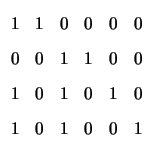
distance no less than d. Figure 1.1 depicts a ternary
non-linear code and a binary linear code.
qn
of dimension k with
the property that any two vectors in the subspace are separated by a Hamming
distance no less than d. Figure 1.1 depicts a ternary
non-linear code and a binary linear code.
![\begin{figure}\centering\subfigure[]%%[Vectors of a ternary non-linear $[n=6,M=3...
...& 1\\
1& 1& 1& 1& 0& 0\\
1& 1& 0& 0& 1& 1\\ \hline
\end{tabular}}
\end{figure}](img37.png) |
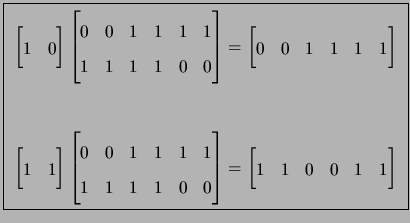
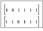
We will typically specify a linear code by its set of basis vectors (also known as generators), which form the rows of a generator matrix G. A parity-check matrix for a linear code is a matrix H with the property that GHT = 0 for some generator matrix G of the code. For example, the linear code in Figure 1.1 has parity-check matrix
Linear codes impose a natural coset-structure on their ambient vector spaces.
Specifically,
given a linear code
![]() , we can say that
two vectors
v1, v2
, we can say that
two vectors
v1, v2![]()
![]() qn are in the same coset if
and only if
qn are in the same coset if
and only if
![]() . Moreover, we can represent each
coset by a coset leader which is arbitrarily chosen among the lowest
weight vectors in a coset. For example, some cosets of the linear code in
Figure 1.1 are:
. Moreover, we can represent each
coset by a coset leader which is arbitrarily chosen among the lowest
weight vectors in a coset. For example, some cosets of the linear code in
Figure 1.1 are:
| C0 | = | {000000, 001111, 111100, 110011} | |
| C1 | = | {000001, 001110, 111101, 110010} | |
| C2 | = | {000011, 001100, 111111, 110000} |
To use an (n, k, d ) binary linear code over
a communications channel, a user would split his input into blocks of
k bits each and encode each block b by multiplying it by the
generator matrix G. The resulting n-bit vector bG is
sent over the channel giving a transmission rate of k/n.
The receiver then decodes the
received error-corrupted vector bG + e to the nearest vector v
in the code. The vector v will be equal to bG as long
as the error e contains no more than
![]() bits.
Figure 1.2
depicts this transmission model.
The type of decoding we have described
is also known as maximum-likelihood decoding because it decodes
to the most likely transmitted input. Several descriptions
of this communications model may be found in [42], [7],
and [4].
bits.
Figure 1.2
depicts this transmission model.
The type of decoding we have described
is also known as maximum-likelihood decoding because it decodes
to the most likely transmitted input. Several descriptions
of this communications model may be found in [42], [7],
and [4].
|
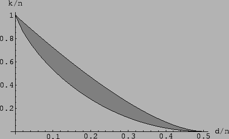
Often when we talk about a family of linear error-correcting codes, we shall be interested in the asymptotic tendency of the code. Specifically, we would like that, as the length n increases, the error-correction capability of the code likewise increases. It has been proven that there exist families of linear codes which achieve the Gilbert-Varshamov bound [42], namely
| (9) |
On the other hand, the McEliece, Rodemich, Rumsey, and Welch [4] provide a well known upper bound on the parameters of linear codes
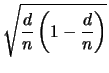 |
(9) |
 |