 ...researching fundamentals of networking and communications
|
Error Control Codes for Data SynchronizationIntroductionThe Reconciliation Problem: Some of the common applications where synchronization plays a vital role are Domain Name Servers (DNS) that constantly have to map new IP addresses to new web pages and also remove records of web pages that are no longer in service. Different DNS servers in a network have to constantly synchronize with each other to maintain consistent data. Another common application that employs synchronization is databases that maintain resources available in a network. Resources are continually added to and taken off from a network. At any given time, any person who has logged into the network needs to know all the available resources and this list should be complete and up to date. Yet another common area where synchronization plays a key role is in the maintaining of bank accounts over distributed databases across a large country. Different servers maintain the same records of the databases across geographically separated locations for faster access of records and these records need to be perfectly in synchronization. Nowadays PDA�s are very common. PDA�s need to synchronize between various devices to update their records. Some of the common methods employed by PDA�s for synchronization are: Slow Sync, where the PDA and a PC or laptop can transfer data back and forth. The record of one device is transferred in its entirety to the other device regardless of whether the other device has a part of the record that is being transferred. Hot Sync, where the two devices can synchronize their data and make updates only on those records that have been updated since the last synchronization. The drawback here is that the same two devices need to be always involved with the synchronization. The overall problem of synchronization can be visualized as, a group of devices, each maintaining a database and each device should keep track of the changes taking place in each of the other devices and present the most up to date information to any application or user. For the sake of analysis, the problem can be formalized as follows: Given a pair of devices or nodes in a network, A and B, each with a set of length-b bit strings (denoted as Sa and Sb), and no a- priori knowledge of the other host set, each host has to determine the mutual differences between the two sets with a minimal amount of communication. Minimality is measured in terms of number of bits transmitted across the link, number of times each host communicates with the other, and computational complexity of the entire reconciliation. This is known as the Set Reconciliation problem. The data represented in each host or device is considered as sets whose elements are chosen from a finite universal set U. Every set S whose elements are taken from U may be associated uniquely with a characteristic vector v(S) of length |U|. The components of the characteristic vector are either a 0 or a 1. The i-th component of the characteristic vector of set S is 1 if and only if the i-th element of the universal set U occurs in the set. For example, the characteristic vector of the set : S={3,5,9} taken over the universal set U=Z24 would be: V(S) = 0 0 0 1 0 1 0 0 0 1 0 0 0 0 0 0 Reconciling two sets involves determining the mutual difference between two such characteristic vectors. Synchronization Issues : Each type of networked device that must synchronize with another, usually is capable of only a select few methods of synchronization depending on the application running on each device. In some cases the bandwidth available to certain devices limits the speed and methods of synchronization. For devices like PDA�s the computational power of the processor is minimal and cannot be expected to perform complex procedures to limit the amount of communication bits or the number of rounds of communication. An optimal synchronization protocol should be capable of synchronizing any two heterogeneous or homogeneous devices with minimum amount of communication bits, minimum computation complexity and minimum number of rounds of communication between the devices.Error Control CodesOverview of Error Correcting Codes Error Correcting Codes are commonly used to transmit data over noisy communication channels. The noisy channel may introduce errors like flipping of bits or deletion or insertion of bits. The simplest form of error correcting codes usually correct errors that are caused by flipping of bits. The general scheme of error correcting code is as follows: The encoder converts a message into a codeword by adding a certain amount of redundancy to the message bits. The method of determining the redundancy bits varies for different schemes of encoding. The encoded message is sent across a noisy channel At the receiver end, the decoder tries to determine the exact message that was sent by making use of the message bits and the redundant bits that were transmitted across the channel. Each coding scheme has certain limitations on the error conditions that can be corrected. The amount of redundant data attached to each packet is pre-determined by the amount of noise that a channel may add to each packet. Error Correcting Codes for Data Synchronization: The data synchronization scheme using error-correcting codes assumes that data on each device is in the form of sets. The elements of the sets are unindexed, meaning that only the content of the individual sets matter and not the relative position of the elements within the set. Each host determines its characteristic vector as described earlier. Each characteristic vector is of length equal to that of a valid code word of the code C. The length of the code word is the value of the maximum allowable element in the set. Each characteristic vector can be thought of as a received code word. These code words could be valid or invalid depending on the values of the data present in each set. The decoding algorithm of the coding scheme when applied to the characteristic vector gives an idea of the distance of the characteristic vector from a valid code word. One very popular and extensively studied coding scheme is the BCH Error Correcting Code. For the purpose of synchronization the BCH code was chosen because of the vast amount of literature available about BCH codes. An implementation of Tornado codes and LDPC codes were also studied to see if they could be applied to the Set-Reconciliation problem.BCH CodesOverview of BCH codes The BCH family of codes is an Error Correcting Code that enables a limited number of errors to be detected and corrected. BCH codes were discovered independently by Bose and Ray Choudhury in 1960 and Hocquenghem in 1959. Basic Concepts The concepts and theories are very much involved with number theory and advanced linear algebra knowledge that are quite abstract. Some definitions: Galois Fields GF(q) is a field with q elements, also called a finite field because there are a finite number (q) of elements. A Primitive Element of GF(q) is an element �a�such that every field element except zero can be expressed as a power of a . Each Galois Field has at least one primitive element. If q = 2m, where m is any integer, the elements of the field can be represented by polynomials whose co-efficients are elements of the field GF(2) i.e 0 and 1. The primitive element of such a field would itself be such a polynomial. The block length of the code is n = 2m-1 The error correcting capability of the code is bounded by t < (2m �1)/2 Encoding: The idea is to create a codeword which contains two parts : a remainder part for checking and the message part. To generate the complete codeword, the data part (the part that is to be encoded) is divided by a generator polynomial to get the remainder part, just as in ordinary polynomial division modulo 2. The number of bits assigned for the remainder is decided by first estimating the probability of error on the channel. The encoding scheme can be summarized in the following steps: Choose the degree m and the corresponding primitive polynomial p(x) and construct Galois Field GF(2m) Obtain a generator polynomial. Determine remainder Left shift data bits by number of bits assigned for remainder. Append remainder to data to get a complete code word. To encode a source message u(X) using a BCH code with generator polynomial g(X), the parity check symbols are found using the formula: b(X) = Xn-ku(X)( mod g(X) ) The encoded code word is : v(X) = Xn-k u(X) + b(X) BCH Decoder Suppose a valid codeword to be : v(X) = v0 + v1X + ��+ vn-1 Xn-1 and the received codeword: r(X) = r0 + r1X + � + rn-1 X n-1 The error pattern is : e(X) = r(X) �vc(X) = e0 + e1X + � + en-1 Xn-1. To determine the error vector, the received code word is passed through the decoding algorithm that is summarized below: First the syndrome set S ={S1, S2, �, S2t} is computed. Each Syndrome is computed as : Si=r(ai) The error locator polynomial s(X) is found using the Berlekamp-Massey algorithm described in the next section. The error location numbers b1 through bnu are found by finding the inverses of the roots of s(X). Once the locations of the errors are known, the received code word can be corrected to obtain the correct code word. BCH codes for Data Synchronization The host that has the most up-to-date data set computes its characteristic vector and determines its syndrome by applying the BCH decoding algorithm. This syndrome is then broadcast to all other hosts on the network that need to be synchronized. Each host calculates their syndromes for their own characteristic vectors. Each host now adds (modulo 2 which is equivalent to XORing) its own syndrome and the syndrome it received The resultant syndrome when decoded determines the error locator polynomial, which indicates the location of errors in the characteristic vector formed by the addition (modulo 2) of the two characteristic vectors.. The error locator polynomial when added (modulo 2 ) to the characteristic vector determined by the target host results in a characteristic vector that exactly resembles the characteristic vector of the host with the most up-to-date data set. The extraction of the set elements from the characteristic vector is a trivial problem. It has to be borne in mind however that the maximum number of differences between the sets is bounded by the error correcting capability of the code.The Berlekamp-Massey AlgorithmThe Berlekamp-Massey algorithm computes the error location polynomial s(X). The main steps involved in the algorithm are: � Initialize the following values: s(X) = 1 l = 0 b(X) = 0 � For m =1 to 2t, do the following: Compute the discrepancy : l d = � siSm-i 0 Where si is the co-efficient corresponding to X i in s(X) If d � 0, do the following: s �(X) = s(X) � dXb(X) If 2l <m , do the following: b(X) = d-1s(X) l = m - l Else (2l � m), do the following: b(X) = X b(X) s (X) = s�(X) Else (d = 0), do the following: b(X) = X b(X) � If the degree of s(X) � l, then more than t errors have occurred and they cannot be corrected.Tornado CodesOverview of Tornado Codes A code C(B) is defined as a set of n message bits and b n check bits that are associated with a bipartite graph B. The graph B has n left nodes and b n right nodes, corresponding to the message bits and the check bits respectively. The encoding consists of computing each check bit as the sum of the bits of its neighbors in B. The encoding time is proportional to the number of edges in B. If the value of a check bit is known and all but one of the message bits associated with that check bit is known, the missing message bit can be found by computing the sum of the check bit and its known message bits.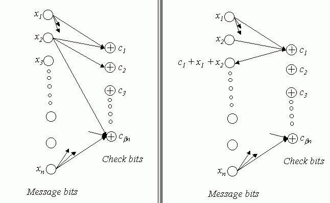 Fig1 Graph representation of one stage of the Tornado Code. (Fig from �Practical Loss-Resilient Codes�, by Michael Luby, Michael Mitzenmacher, Amin Shokrollahi, Daniel Spielman and Volker Stelmann) Encoding and decoding are simple XOR operations on bits or packets. The total decoding time is proportional to the number of edges in the graph. From the above diagram it is clear that at most one message bit that contributes to a particular check bit or the check bit itself, can be lost if the code is to be recovered. To produce codes that are more loss � resilient, the basic structure is cascaded to form the cascaded code C(B). The first structure produces b n check bits for the original n message bits and at the next stage a similar structure is used to produce b 2 n check bits for the b n check bits. At the final stage a conventional loss resilient code such as Reed- Solomon or BCH code is used. The final code would resemble the following diagram: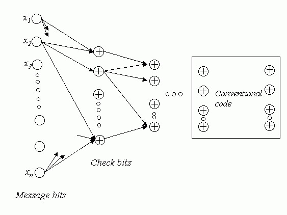 Fig2 Graph representation of the complete code. (Fig from �Practical Loss-Resilient Codes�) The number of stages and the basic structure of the bipartite graph involve a very complicated design procedure based on differential equations that are beyond the scope of this project. An implementation of the Tornado code developed by Jeffrey Considine was used to explore the possibility of the use of these codes in data synchronization.LDPC CodesOverview of LDPC Codes: LDPC codes or Low-Density Parity-Check Codes are a class of codes where each code is specified by a parity-check matrix with the following properties: � Each column contains a small fixed number j>= 3 of 1�s and � Each row contains a small fixed number k>j of 1�s. � A majority of the entries in the matrix are 0�s An (n,j,k) low-density code is a code of block length n with a matrix as shown below: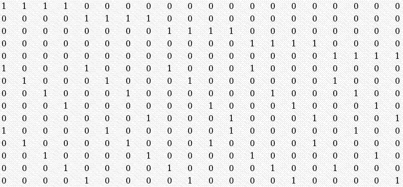 In the above code N=20, j=3, k=4. (Matrix from �Low-Density Parity-Check Codes�, by R.G. Gallagher.
The encoding procedure is similar to that of any linear code, where the message bits are multiplied by a generator matrix to produce a code word. Each parity check matrix has a generator matrix associated with it and if one is given, the other can be easily determined.
Decoding:
There are two basic decoding schemes for the LDPC codes.
In the first scheme, the decoder computes all parity checks and then changes any digit that is contained in more than some fixed number of unsatisfied parity- check equations. Using these new values, the parity checks are recomputed, and the process is repeated until the parity checks are all satisfied.
In the second scheme an algorithm known as the �sum-product� algorithm is used which is similar to the �belief-propagation algorithm� used in networks.
Information about each bit of the codeword derived from the received data is expressed as a probability ratio, the probability of the bit being 1 divided by the probability of the bit being 0. The probability ratios will be adjusted to take account of information obtained from other bits along with the requirement that the parity checks be satisfied.
The algorithm alternates between recalculating the probability ratios for each check.
In the above code N=20, j=3, k=4. (Matrix from �Low-Density Parity-Check Codes�, by R.G. Gallagher.
The encoding procedure is similar to that of any linear code, where the message bits are multiplied by a generator matrix to produce a code word. Each parity check matrix has a generator matrix associated with it and if one is given, the other can be easily determined.
Decoding:
There are two basic decoding schemes for the LDPC codes.
In the first scheme, the decoder computes all parity checks and then changes any digit that is contained in more than some fixed number of unsatisfied parity- check equations. Using these new values, the parity checks are recomputed, and the process is repeated until the parity checks are all satisfied.
In the second scheme an algorithm known as the �sum-product� algorithm is used which is similar to the �belief-propagation algorithm� used in networks.
Information about each bit of the codeword derived from the received data is expressed as a probability ratio, the probability of the bit being 1 divided by the probability of the bit being 0. The probability ratios will be adjusted to take account of information obtained from other bits along with the requirement that the parity checks be satisfied.
The algorithm alternates between recalculating the probability ratios for each check.
Implementation, Results and ConclusionsBCH Codes:Implementation Two approaches were taken towards implementing the BCH decoder. In the first approach, a look up table was created that stored all the different exponents of the primitive element a. In the second approach, the required exponent values of a were calculated at run time. All coding was done in the �C� programming language on Linux platform. Results of the two approaches: The graphs below show the performance of both the approaches for various parameters.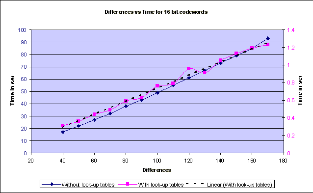 Graph1:The graph above shows the variation of the reconciliation time with respect to number of differences between the sets. The dotted line is a linear fitting for the values obtained with the implementation that used look-up tables. The axes are colored according to the respective plots they refer to. 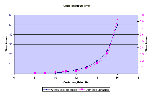 Graph 2: The graph above shows the variation of the reconciliation time with respect to the length of the codewords. Comparison between performance of Characteristic Polynomial Interpolation scheme and Error Correcting Code (BCH Code) scheme: The table below lists the time taken in milliseconds to synchronize two sets with 16 bit elements for various number of differences between them.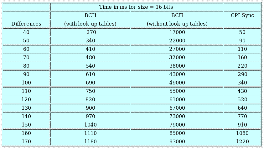 Table 1 The graph below shows a plot of the data from the table: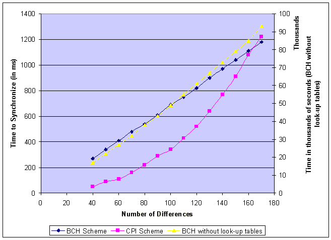 Graph 3: Comparison of BCH scheme and CPI scheme for 16 bit vectors. Note: All data collected by running the code on a PIII with 196 Mb of RAM, running Linux (Red Hat 7.0) Conclusions drawn from the BCH Error-Correcting-Code Set-Reconciliation scheme: From Graph1, it appears that the reconciliation time for the BCH scheme with and without look-up tables grow linearly as the number of differences increase. The amount of memory required by the BCH scheme when implemented with a look up table is, however, an exponential function of the length of the code. (Q(2n)). As is evident from Graph1, there is a significant difference in the time taken by the two approaches, a difference of almost 69 seconds for 130 differences between the sets. From Graph 3, it is also clear that for small differences between the sets, CPI synchronization consumes less time but as the number of differences between the sets increases, the BCH scheme, increases almost linearly but the CPI synchronization scheme increases quadratically. The only drawback of the BCH scheme is that the constants involved in the running time are relatively large. And even between the two approaches to the BCH scheme, the scheme with look-up tables has a much smaller constant when compared to the approach without look-up tables. From Graph2, it is clear that the running time of the BCH scheme, in both approaches, is exponential in the length of the codeword. This fact affects the constant term involved in the running time for a given length of codeword. The maximum size of the look � up table is bounded by the amount of memory available and the maximum value that an integer variable can assume. This is because the array index has to be an integer. The large constants involved in the scheme without look-up tables makes it a non-practical scheme for set reconciliation. Also, the amount of memory that is required for the scheme with look-up tables is not practical when synchronizing large databases whose contents may require representation with up to 512 bits. A simple analysis of the BCH decoding scheme reveals that the maximum amount of time (more than 99% of the total running time) is taken up by the final stage of the decoding process � the Chien Search. Each bit of the vector has to be examined to check if it is in error. If the data is represented by 16 bits, the length of the characteristic vector would be 216 and each bit of this vector has to be checked for error in the Chien Search. This leads to the possibility of usage of this scheme in scenarios where either only deletions or only insertions take place. If we knew before hand that a particular server is going to make only deletions in its data set, we would just need to examine each bit of the characteristic vector on the client that is �set� to see if it is in error. Again, if we know before hand that the server is going to make only insertions, we can model these insertions as deletions. We can check all the �unset� bits in the characteristic vector on the client to see if they are in error. The running time of such an operation would be dependent only on the number of entries in the set. Again, this scheme would be useful only if the data set on the server has a small number of initial entries on which insertions are performed or if it has a very large number of entries on which deletions are performed. Tornado Codes: Implementation issues and conclusions: Tornado codes are difficult to implement, as there isn�t much documentation available on the codes. Designing good graphs for the codes involves complex differential equations. The code that was used in the project was of very low rate (less than 1/2). The basic idea behind using error-correcting codes for the Set Reconciliation problem was to use the redundant bits in an error-correcting code to synchronize two hosts. In this implementation the number of redundant bits exceeded the number of message bits and so, wasn�t really practical to apply it to the Set � Reconciliation problem. LDPC Codes: Implementation issues and conclusions: An implementation of LDPC codes developed by Radford McNeal2 and David MacKay3 was used in the study. The software is capable of simulating memoryless channels, including Binary Symmetric Channels and Additive White Gaussian Noise Channels. Results: The code wasn�t s able to decode some arbitrarily random vectors. When synchronizing databases that contain critical information, it is absolutely necessary that the two hosts reflect the same data. The fact that the LDPC codes cannot correct all possible errors, however, make it a bad choice for application to the Set Reconciliation problem. Although the results of this project clearly indicate that Error Correcting Codes can be used for the Set Reconciliation problem, most of the codes available right now are not well suited for this purpose.Downloads and Links* Downloads:* BCH Set reconciliation scheme with look-up tables : Download BCH Set reconciliation scheme without look up tables : Download Project Report in pdf LDPC-code software developed by Radford McNeal and David MacKay NTL - Victor Shoup's Number Theory Library Papers: "Connections between Data Reconciliation and Generalized Error Correcting Codes "[ Ari Trachtenberg, Mark Karpovsky, Lev Levitin] " Set Reconciliation with Nearly Optimal Communication Complexity " [Yaron Minsky, Ari Trachtenberg, Richard Zippel] "Practical Loss Resilient Codes " [Michael Luby, Michael Mitzenmacher, Amin Shokrollahi, Daniel Spielman, Volker Stemann] Links: Lab of Networking and Information Systems at BU . Prof. Trachtenberg's website. The Error Control Codes (ECC) Home Page David MacKay's Gallager code resourcesReferences1. �Error Control Coding� [Shu Lin, Daniel J. Costello Jr.] 2. �Data Verification and Reconciliation with Generalized Error-Control Codes.� [Mark G. Karpovsky, Lev B. Levitin, Ari Trachtenberg] 3. �Set Reconciliation with Nearly Optimal Communication Complexity.� [Yaron Minsky, Ari Trachtenberg, Richard Zippel] 4. �Efficient Reconciliation of Unordered Databases.� [ Yaron Minsky, Ari Trachtenberg] 5. �Error Correcting Codes.� [ Peterson and Weldon] 6. �The Theory of Error-Correcting Codes�[MacWilliams and Sloane] 7. �Coding and Information Theory.� [Steven Roman] 8. �A First Course in Coding Theory.� [Raymond Hill] 9. �Practical Loss Resilient Codes.� [Michael Luby, Michael Mitzenmacher, Amin Shokrollahi, Daniel Spielman, Volker Stemann] 10. �Low-Density Parity-Check Codes.� [R. Gallagher] 11. �The Error-Correcting Codes Page.� [ http://www.csl.sony.co.jp/person/morelos/ecc/codes.html ] |
|
Photonics Building, Room 413
8 St Mary's Street,
Boston MA 02215
Initial web site created by Sachin Agarwal (ska@alum.bu.edu), Modified by Weiyao Xiao (weiyao@alum.bu.edu), Moved to TWiki backend by Ari Trachtenberg (trachten@bu.edu). Managed by Jiaxi Jin (jin@bu.edu).