


Next: System Model
Up: PDA Synchronization
Previous: CPISync
Contents
Deterministic CPISync
Synchronization is done on two sets of
similar data sets held on two different devices. By
similar we mean that most of the records in the data sets
are identical. Three types of updates may occur in databases - an
addition of a record, a deletion of a record or a modification of
a record, each introducing a difference.
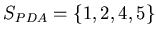
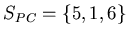
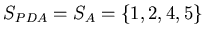
Consider a set  , a data set on the PDA and a similar set
on the PC, namely
, a data set on the PDA and a similar set
on the PC, namely  . and were probably
derived from the same identical set (a previous synchronization
and subsequent independent updates on the hosts for example). For
simplicity we consider sets of integers. For example
. and were probably
derived from the same identical set (a previous synchronization
and subsequent independent updates on the hosts for example). For
simplicity we consider sets of integers. For example
 and
and
 . The objective of an
efficient synchronization routine is to determine the set
. The objective of an
efficient synchronization routine is to determine the set
 and install this set
  in the PDA and the PC in the least possible time, using the least
amount of communication and computation.
CPISync first constructs a characteristic polynomial for each of
the data sets it is reconciling which is simply a univariate
polynomial whose factors are the elements in of the data set.
These characteristic polynomials is sampled at
in the PDA and the PC in the least possible time, using the least
amount of communication and computation.
CPISync first constructs a characteristic polynomial for each of
the data sets it is reconciling which is simply a univariate
polynomial whose factors are the elements in of the data set.
These characteristic polynomials is sampled at
 sample points. The PDA sends these evaluations to the PC which
calculates rational function evaluations by taking the ratios of
the evaluations of the characteristic polynomials at the same
sample points and interpolating a rational function
sample points. The PDA sends these evaluations to the PC which
calculates rational function evaluations by taking the ratios of
the evaluations of the characteristic polynomials at the same
sample points and interpolating a rational function  fitting
the points. The factors of the numerator and denominator of
give the different (missing) set data.
We now explain the CPISync Algorithm in detail by means of the
example given above. Figure 3.1 outlines the
steps of the algorithm which are itemized below.
fitting
the points. The factors of the numerator and denominator of
give the different (missing) set data.
We now explain the CPISync Algorithm in detail by means of the
example given above. Figure 3.1 outlines the
steps of the algorithm which are itemized below.
Figure 3.1:
CPISync Algorithm - a simple example showing
interpolation based synchronization
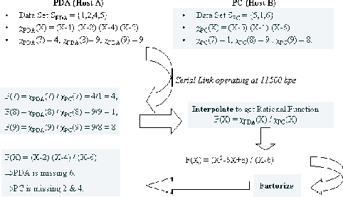 |
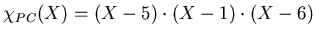
- The PDA calculates the characteristic polynomial function
from its data set . A characteristic polynomial function
has all the data set elements as its factors, as is shown in
figure 3.1. For example, for
 , the characteristic polynomial function
 . This is the
`signature' of the information contained in the data set. The PC
also calculates the characteristic polynomial function for its own
data set =
. This is the
`signature' of the information contained in the data set. The PC
also calculates the characteristic polynomial function for its own
data set =
 ;
;
 . Note that the characteristic
polynomials are always monic, i.e., the highest degree term of the
polynomial has coefficient
. Note that the characteristic
polynomials are always monic, i.e., the highest degree term of the
polynomial has coefficient  .
.
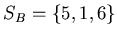
- The characteristic function on the PDA is then `sampled' at
some pre-selected random sample points. In our example, these are
 . The number of sample points has to be at least equal
to the number of differences in the system which explains the need
to know an upper bound
on the number of differences
in the system.
. The number of sample points has to be at least equal
to the number of differences in the system which explains the need
to know an upper bound
on the number of differences
in the system.
- The sampled characteristic polynomial function values of the
PDA are transferred to the PC from the PDA. This almost completes
the PDA's job, it is now up to the computationally stronger PC to
do the remaining steps of the reconciliation synchronization. In
Figure 3.1 the shaded text indicates the
computation performed on the PC: this is the asymmetric capability
of the CPISync algorithm.
- The PC calculates rational function instantiations by
dividing each sample point evaluation of the PDA's characteristic
polynomial function with its own characteristic polynomial
function's evaluation at that same sample point, ending up with
2-tuples of (sample point, rational function
evaluation).
- These 2-tuples are then interpolated to obtain the
rational function
 . This rational function is of the type
 where
where  and
and  are (unreduced)
polynomials with coefficients in the finite field
are (unreduced)
polynomials with coefficients in the finite field  (in our
example). and are divided with their GCD to obtain
an irreducible polynomial of the form
(in our
example). and are divided with their GCD to obtain
an irreducible polynomial of the form
 . The sum
of the degrees of
. The sum
of the degrees of  and
and  equal the total number of
differences between the data sets and .
equal the total number of
differences between the data sets and .
- and are separately factored yielding the
differences the PDA and the PC are missing respectively. The
factors of are sent to the PDA to update its data set,
while the factors of are used by the PC to update its own
data set and incorporate the new data from the PDA that it had
been missing.
Note that the last step is the most simplistic scenario. There
might be instances of conflicts (see section 2.1)
which would need to be dealt with separately.
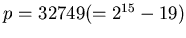
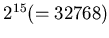
There are some subtleties that need to be explained at this point.
The first is the use of finite field arithmetic to limit the size
of the characteristic polynomial evaluations because their
calculation involves evaluating a product of factors which grows
very rapidly. We have used  for the PC-PDA
synchronization, which gives us a 15-bit space for the
mathematical operations. One bit out of these is used for the
sample points, which are discussed next.
for the PC-PDA
synchronization, which gives us a 15-bit space for the
mathematical operations. One bit out of these is used for the
sample points, which are discussed next.
Figure 3.2:
The finite field space is divided into two regions, one
for sample points and the other for data
points
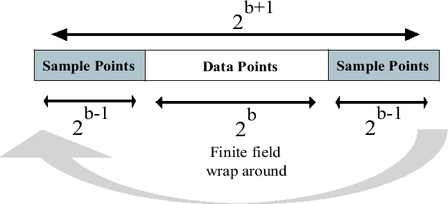 |
There are two things that need to be explained about the choice of
the sample points. The sample points need to be separate from
the data points in the set. This is because otherwise, the
characteristic polynomial of the corresponding data set will
evaluate to 0 in step  . In our example
(Figure 3.1), if we selected as a sample
point, the characteristic polynomial evaluation
. In our example
(Figure 3.1), if we selected as a sample
point, the characteristic polynomial evaluation
 . A bad choice may result
in a division-by-zero error in step
. A bad choice may result
in a division-by-zero error in step  of the algorithm.
Since we do not know a priori the number of differences in the
data to be reconciled, we increase the size of the finite field by
approximately bit. One bit provides adequate space to
accommodate the sample points because for
of the algorithm.
Since we do not know a priori the number of differences in the
data to be reconciled, we increase the size of the finite field by
approximately bit. One bit provides adequate space to
accommodate the sample points because for  bit data, there can
be a maximum of
bit data, there can
be a maximum of  differences between any two data sets and
CPISync requires at least as many sample points as there are
differences. This concept is shown in
figure 3.2. The idea here is to pick the sample
points from a separate `region' of the number line than
the data points, eliminating the possibility of a `collision'
between the data and sample points.
The specific choice of the region of sample points in
Figure 3.2 is because choosing sample points
symmetrically over the 0 point speeds up calculations in the
Gaussian elimination involved in interpolation in step of the
algorithm described above. Symmetric sample points (such as
differences between any two data sets and
CPISync requires at least as many sample points as there are
differences. This concept is shown in
figure 3.2. The idea here is to pick the sample
points from a separate `region' of the number line than
the data points, eliminating the possibility of a `collision'
between the data and sample points.
The specific choice of the region of sample points in
Figure 3.2 is because choosing sample points
symmetrically over the 0 point speeds up calculations in the
Gaussian elimination involved in interpolation in step of the
algorithm described above. Symmetric sample points (such as
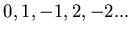 ) help in making the Gaussian elimination faster
by making it simple to get many zeros in the matrix while solving
for the coefficients of the rational function, thus speeding up
Gaussian elimination. This is particularly important because as we
will see later, most of the latency arises from this Gaussian
elimination. Note that exact symmetry about 0 is possible only
for an odd number of sample points.
A second point of interest to mention here is the choice of the
finite field. We have used
) help in making the Gaussian elimination faster
by making it simple to get many zeros in the matrix while solving
for the coefficients of the rational function, thus speeding up
Gaussian elimination. This is particularly important because as we
will see later, most of the latency arises from this Gaussian
elimination. Note that exact symmetry about 0 is possible only
for an odd number of sample points.
A second point of interest to mention here is the choice of the
finite field. We have used  where
where  is a prime
number. For the Palm PDA, the word size is 16 bits. We carefully
chose
is a prime
number. For the Palm PDA, the word size is 16 bits. We carefully
chose
 . This is the largest prime
number less than
. This is the largest prime
number less than
 .
In case the records are variable length strings, they may be
hashed into fixed small length hashes to be used as the data set
elements that are reconciled using CPISync. The difference
information in terms of hashes reported by CPISync may then be
transformed into information about the corresponding differing
strings using a reverse table lookup. We have avoided the issues
of hashing by restricting our record database entries to 15-bit
integers. We note that, in practice, the hashing operation needs
to be performed only once per entry, at the time that the entry is
added to the data set, thus the complexity of the hashing is not a
bottleneck for synchronization. By restricting entries to 15 bits,
we have also avoided the issues of multiple-precision arithmetic
on the PDA.
.
In case the records are variable length strings, they may be
hashed into fixed small length hashes to be used as the data set
elements that are reconciled using CPISync. The difference
information in terms of hashes reported by CPISync may then be
transformed into information about the corresponding differing
strings using a reverse table lookup. We have avoided the issues
of hashing by restricting our record database entries to 15-bit
integers. We note that, in practice, the hashing operation needs
to be performed only once per entry, at the time that the entry is
added to the data set, thus the complexity of the hashing is not a
bottleneck for synchronization. By restricting entries to 15 bits,
we have also avoided the issues of multiple-precision arithmetic
on the PDA.
Figure 3.3:
The overall scheme of the PC-PDA
synchronization system
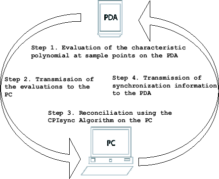 |
Figure 3.3 shows the high level scheme of the PDA-PC
synchronization. The thing to note here is that the transfer of
data (indicated by the arrows) is typically through a slow link.
In the case of a Palm PDA, the transfer is through a serial cable
or IrDA (Async Serial-IR 9600-115.2kb/s) [28]. Newer PDAs
have USB [18] and Ethernet connectivity. These technologies
are substantially faster than serial links, though newer PDAs
often run more data intensive applications, leaving the problem of
slow data transfer between the PDA and the PC network intact, as
was shown in Figure 2.5.
Figure 3.3 indicates that the total communication
between the PDA and the PC is simply the transmission of the
characteristic polynomial function evaluations from the PDA to the
PC (there are
such evaluations). After the
reconciliation is complete, the number of data set elements the
PDA is missing (
at worst) are transferred back to
the PDA. Thus taken totally, the number of data elements
transferred is O(
), irrespective of the sizes of the
data sets on the PDA and the PC.
Subsections
Next: System Model
Up: PDA Synchronization
Previous: CPISync
Contents
Sachin Kumar Agarwal
2002-07-12