Results

We ran the CPISync and Slowsync protocols on the PC-PDA synchronization system for various set sizes - varying from sets of $100$ elements to sets of $10000$ elements with differences varying from 0 to more than $1200$ for these data sets. We timed the total latency of the synchronization as the sum of the communication time (time taken to transfer data from the PDA to the PC) and the computational time (time taken to reconcile the data sets), ignoring the time to upload data from the PC back to the PDA since this is identical for both the protocols. 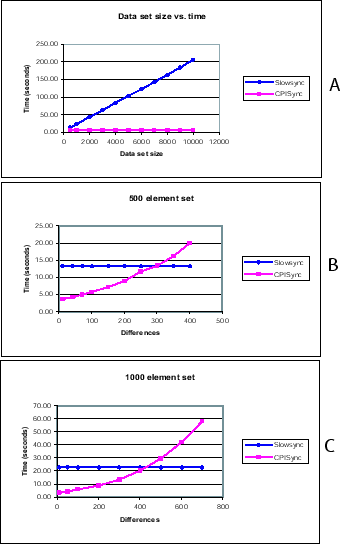Figures 3.6 and 3.7 show some of the data we collected. The values given are averages over $10$ trials of identical experiments.

Figure 3.6: (A) highlights the superiority of CPISync over Slowsync by showing that Slowsync does not scale with increasing number of elements in a data set and a fixed number of differences. The next two graphs show the comparison the latency of CPISync and Slowsync for (B) $500$ and (C) $1000$ element sets and varying differences.

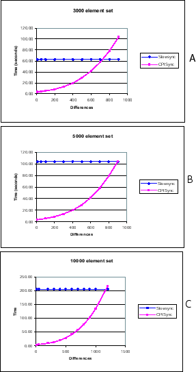
Figure 3.7: These three graphs show the comparison the latency of CPISync and Slowsync for (A) $3000$, (B) $5000$ and (C) $10000$ element sets and varying differences.

Figure 3.5 (a) depicts the superior scalability of CPISync over Slowsync. In this figure we have plotted the time used by each synchronization scheme as a function of data set size for a fixed number of differences between data sets. It is clear from the resulting graphs that Slowsync is markedly non scalable: the time taken by Slowsync increases linearly with the size of the data sets. CPISync on the other hand is almost independent of the data set sizes. Comparing Figure  2.3 to Figure 3.5 (a) we observe that the qualitative behavior of CPISync is similar to that of Fastsync. The remarkable property of CPISync is that it can be employed for any synchronization scenario, regardless of context, whereas Fastsync is employed only when the synchronization took place between the same PC and the same PDA.

Table 3.1: Threshold values at which CPISync takes the same time as Slowsync.

Data set Size	Differences
100	161
250	175
500	253
1000	431
2500	620
3000	727
5000	899
10000	1177

In figure 3.5 (b), we compare the performance of CPISync to Slowsync for data sets with fixed sizes but increasing number of differences. As expected, CPISync performs significantly better than Slowsync when the two synchronizing data sets do not differ by much. However as the number of differences between the two data sets increase, the computational complexity of CPISync becomes significant. Thus, there exists a threshold where wholesale data transfer (Slowsync) becomes a faster method of synchronization; this threshold is a function of the data set sizes as well as the number of differences between the two data sets. For the $10,000$ record sets depicted in the figure, this threshold corresponds to roughly $1200$ differences. By preparing graphs like Figures 3.6 and  3.7 for various different set sizes, we are able to produce a regression with coefficient of determination^3.1 [33] almost $1$ that analytically models the performance of Slowsync and CPISync. The resulting threshold values are listed in Table  3.1. The regression for Slowsync is obtained using Maple by fitting the data to a linear function that depends only on the data set size, where as for CPISync the regression is obtained by fitting the data to a cubic polynomial using Maple that depends only on the number of differences. Note that in a PDA application like an address book or memo, changes between concurrent synchronization typically involve only a small number of records. For such applications, CPISync will usually be much faster than Slow Sync. In Table 3.2, we show the fitted cubic polynomials generated using Maple corresponding to $100$, $250$, $500$, $1000$, $3000$, $5000$ and $10000$ element data sets for the total time(latency) with parameter $m$ (differences). It is interesting to note that for a small data sets (and consequently small differences), it is the communication time which seems to dominate and the cubic fit is not good, whereas for sets of size $1000$ or more, the cubic computational complexity dominates the total latency. The communication time is dependent on the operating systems on the PDA and the PC and there was a high level of inconsistency observed in the timing (of the order of $\pm 30\%$) even though all these results have been averaged out over $10$ trials. In the table, we see there is an overhead of about $3.3$ seconds (constant term coefficient) which corresponds to the setup time of the protocol and other operating system overheads. For bigger size sets ($\geq 1000$), it is interesting to note from Table 3.2 that the highest order (cubic) coefficient is almost the same irrespective of the number of elements in the set. This again shows that CPISync is not dependent on the size of the data set. In fact, for big data sets with considerable differences, the latency may be represented by any one of the polynomials in Table 3.2, since for large values of $m$ the cubic term dominates the value of the latency. We shall use this fact to model an optimal Probabilistic scheme in section 3.3.

Table 3.2: Fitted polynomials $P(m)$ for CPISync running time for various data set sizes.

Data set Size	Fitted Cubic Polynomial
100	$-3.18573E-06m^3+5.41161E-04m^2+2.66366E-03m+3.33124$
250	$1.05747E-06m^3-2.45622E-04m^2+3.36804E-02m+3.23576$
500	$6.28175E-08m^3+2.70934E-05m^2+2.02042E-02m+3.33711$
1000	$1.01182E-07m^3+7.74547E-06m^2+2.32522E-02m+3.13590$
3000	$8.79353E-08m^3+2.59495E-05m^2 +1.63701E-02m+3.45446$
5000	$9.76246E-08m^3+1.37409E-05m^2+2.02848E-02m+3.43659$
10000	$1.03861E-07m^3+4.79533E-06m^2 +2.26613E-02m+3.40529$

The implementation of CPISync described here requires the knowledge of a tight upper bound $\overline{m}$, on the number of differing entries. One simple method for obtaining such a bound involves having both hosts $A$ and $B$ count the number of modifications to their data sets since their last synchronization. The next time the hosts synchronize, host $A$ sends to host $B$ a message containing its number of updates, denoted $\overline{m}_A$. Host $B$ uses its own value $\overline{m}_B$ to compute $\overline{m} = \overline{m}_A + \overline{m}_B$ which is the upper bound on the total number of differences between the two hosts. Clearly, this bound $\overline{m}$ will be tight if the two hosts have performed updates to mutually exclusive records. However, they may be completely off if the hosts have performed exactly the same updates to the same records in their databases. This may happen if, prior to synchronization, both hosts A and B synchronized with a third host $C$. Another problem with this method is that it requires maintaining separate information for each host with which synchronization is performed; this may not be reasonable for large networks. Thus the simple method just described will be rather ineffective for some applications. In the next section we describe a probabilistic scheme that can determine a much tighter value of $\overline{m}$. This result is of fundamental importance as it means that, in a general setting, both the communication and computational complexities of CPISync depend mostly on $\overline{m}$.